Optimization under a budget that can actually run out

Bayesian optimization answers one question: given everything measured so far, what should be measured next? It is the standard tool when each measurement is expensive, which describes a laboratory experiment, a long training run, or any instrument that can only do one thing at a time.

Almost all of the published work on it counts iterations. Twenty evaluations, fifty, a hundred. A real laboratory does not have an iteration budget. It has instrument hours, reagents and booked slots, and different experiments cost different amounts. This project rebuilt the loop around that fact.

Industrial R&D. I own this project end to end: problem framing, the policy designs, the harness architecture, the evaluation methodology, and the handover documentation. The implementation, the instrument data and the internal results belong to my employer and are not published here. The mathematics below is standard and comes from the public literature, cited at the end.

The standard formulation
What breaks when evaluations have prices
The design
A constraint the literature mostly ignores
Engineering
A negative result worth reporting
Scope and limitations
References

The standard formulation

We want to minimise a function \(f\) we cannot write down and can only sample, one expensive evaluation at a time:

\[x^{\star} \;=\; \arg\min_{x \in \mathcal{X}} f(x)\]

Bayesian optimization does this in two moves.

Build a surrogate. Place a Gaussian process prior over \(f\), so that after \(n\) observations the model gives a predicted mean \(\mu_n(x)\) and a standard deviation \(\sigma_n(x)\) at every untried point. The standard deviation is the useful part: it says where the model does not know.

Choose where to look next by maximising an acquisition function. The common choice is expected improvement, the expected amount by which a new point beats the best value seen so far \(f^{+}\):

\[\mathrm{EI}(x) \;=\; \mathbb{E}\big[\max(f^{+} - f(x),\, 0)\big]\]

which for a Gaussian posterior has a closed form in terms of \(\mu_n\), \(\sigma_n\) and the normal density and distribution functions. Maximising it balances exploiting places the model thinks are good against exploring places it is unsure about.

Then evaluate at \(x_{n+1} = \arg\max_x \mathrm{EI}(x)\), add the observation, refit, repeat.

What breaks when evaluations have prices

Nothing above knows what anything costs. Introduce a cost function \(c(x) > 0\), the price of evaluating at \(x\), and two problems appear immediately.

One: the wrong thing is being optimised. Suppose method A reaches a good value in 30 evaluations and method B takes 45. A wins the usual plot. But if A systematically proposes the expensive settings and B the cheap ones, B may reach the same value for half the spend. On the axis that matches the real constraint, B is better. On the axis in the paper, A is.

The established fix is to normalise by cost. Snoek and colleagues proposed expected improvement per unit cost:

\[\mathrm{EIpu}(x) \;=\; \frac{\mathrm{EI}(x)}{c(x)}\]

which prefers a cheap, moderately informative experiment over an expensive, slightly more informative one. This is well known and over a decade old.

Two, and this is the part that is usually skipped: a campaign can fail to finish. Let \(B\) be the total budget and \(S_n = \sum_{i \le n} c(x_i)\) what has been spent. Near the end of a campaign the remaining budget \(B - S_n\) is small, and the acquisition function, which knows nothing about money, happily proposes the most informative experiment available. That experiment may be unaffordable.

Every available response is bad. Run it anyway and overspend. Refuse it and watch the loop propose the same point again. Fall back to something arbitrary. Stop early with budget unspent.

So “how well did the policy do?” is not a well-formed question. It has two parts: what did it achieve, and did it finish inside its budget at all. A policy with excellent final regret that rarely finishes inside its budget is not a good policy. It is one you cannot deploy.

The design

The response is to make affordability structural rather than something checked afterwards.

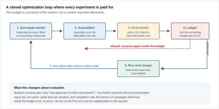
The loop. A proposal is priced before it is accepted, and the ledger can refuse it. The dashed return path is the part most formulations leave out.

A fitted cost model. \(c(x)\) is estimated from real instrument runs rather than assumed. This matters more than it sounds: because the fitted model is a closed form, the affordable set is known exactly before anything is spent.

A ledger. It tracks what has been spent, what remains, and refuses any proposal it cannot pay for. Unglamorous, and it is the component that makes every number downstream honest.

A constrained acquisition step. Not “maximise EI, then check the price” but

\[x_{n+1} \;=\; \arg\max_{x \,\in\, \mathcal{X}_{\text{aff}}} \mathrm{EI}(x), \qquad \mathcal{X}_{\text{aff}} \;=\; \{\, x \in \mathcal{X} \;:\; c(x) \le B - S_n \,\}\]

The difference between these two shows up precisely at the end of a campaign, which is where the behaviour matters. Because \(c\) is a closed form, \(\mathcal{X}_{\text{aff}}\) can be imposed inside the optimization rather than used to reject afterwards.

The harness carries a family of proposal policies, both budget-aware and budget-blind, interchangeable acquisition optimizers, and several benchmark problems, so that the comparisons below are like for like.

A constraint the literature mostly ignores

The total budget is not the only limit. A real instrument is booked in slots, so there is a cap on what a single experiment may consume, separate from what the campaign may consume in total:

\[c(x) \;\le\; c_{\max} \quad \text{for every } x\]

This is a restriction of the problem, not a new policy: it shrinks \(\mathcal{X}\) before any optimization happens. It is also easy to miss, and it changes which policies win, because a policy that earns its advantage by occasionally proposing one very expensive and very informative experiment cannot do so under a slot cap.

Engineering

This is the project I would point to if someone wanted to see how I build software rather than how I design algorithms.

Architecture decision records. Every significant choice has a written record of what was decided, why, and what evidence would reverse it. Six months later this is the difference between a system you can change and one you can only replace.

A reproducibility command. One invocation re-derives every committed figure from the committed data records behind it. A figure that no longer follows from its data becomes a build failure rather than something a colleague notices in a meeting.

A handover document written around a single question: what must a new engineer know on day one in order not to break something or publish a wrong number? I have come to think this is the most useful document in a research repository.

Statistical discipline. A stated detection floor beside every comparison, results over many seeds rather than one, and a count of how many seeds an effect held on. Without a detection floor a small improvement cannot be distinguished from noise, and the reader has no way to tell which they are looking at.

A negative result worth reporting

The natural next idea is non-myopia. Expected improvement optimises the next evaluation only. If three more are affordable, should the loop not plan all three, perhaps spending something cheap and informative now to enable a better choice later?

The fully non-myopic problem is a dynamic program over the remaining budget, and greedy EI is its one-step approximation. In theory looking further ahead is clearly better.

In practice the lookahead costs real compute, it compounds surrogate error over the horizon, and only the two-step version is tractable. So it was built and measured rather than assumed, as its own pre-registered arm with a stated detection floor, and the write-up records the mechanism behind the outcome rather than only the verdict. The internal numbers are my employer’s.

I would rather be the person who measures a sophisticated method and reports what the measurement says than the person who ships it because it ought to work. Deciding not to adopt something, with the evidence attached, saves more engineering time than most positive findings do.

Scope and limitations

Single-objective, one proposal per decision, CPU only. Deliberate limits, written down, so that nobody reads the results as claims about multi-objective or parallel settings.
The cost model is fitted, so it has error. The affordable set is exact with respect to the model, not with respect to the instrument.
The real-instrument grounding rests on a limited number of scans, not a large campaign.
Synthetic and single-instrument. Nothing here speaks to multi-instrument scheduling, which is a different and harder problem.

References

Practical Bayesian Optimization of Machine Learning Algorithms. Jasper Snoek, Hugo Larochelle, Ryan Adams. NeurIPS 2012. Introduces expected improvement per unit cost, the starting point for every cost-aware variant.
Taking the Human Out of the Loop: A Review of Bayesian Optimization. Bobak Shahriari, Kevin Swersky, Ziyu Wang, Ryan Adams, Nando de Freitas. Proc. IEEE, 2016. The standard survey of the formulation in the first section.
Bayesian Optimization with a Finite Budget: An Approximate Dynamic Programming Approach. Remi Lam, Karen Willcox, David Wolpert. NeurIPS 2016. Poses the finite-budget problem as a dynamic program, which is what the two-step lookahead approximates.
Gaussian Processes for Machine Learning. Carl Rasmussen, Christopher Williams. MIT Press, 2006. The surrogate model underneath all of it.

Bayesian optimization that has to pay for its experiments