Cutting search cost in computer-aided synthesis planning
A learned cost-to-go heuristic for retrosynthetic search. Reordering candidate reactions by their remaining distance to purchasable materials raises the solve rate at unchanged per-step compute. Industrial R&D project, owned end to end.
Cost-to-go guidance for retrosynthetic search
A chemist who wants to make a molecule needs a route: a sequence of reactions starting from materials that can actually be bought. Software can propose those routes, and the hard part is not chemistry but search. The number of possible reaction sequences grows so fast with depth that a planner must discard almost every candidate it generates, and if it discards the wrong ones it returns nothing at all.
This project asked a narrow question: can the planner be told where to look, without being given more compute? The answer turned out to involve reusing a quantity the planner already computes.
Industrial R&D. I own this project: problem framing, algorithm design, benchmark construction, evaluation design, and the write-up. I am first author on the resulting conference abstract. The implementation, the internal datasets and the full numbers belong to my employer and are not published here. Everything below is either the published literature or a description of how the work was run, which is the level of detail I can share. The mathematics in this page is from public papers, cited at the end.
Contents
- The problem, stated precisely
- Why the cost explodes
- The quantity that was already there
- What I did with it
- Designing an evaluation that cannot flatter itself
- What was found
- Limitations
- References
The problem, stated precisely
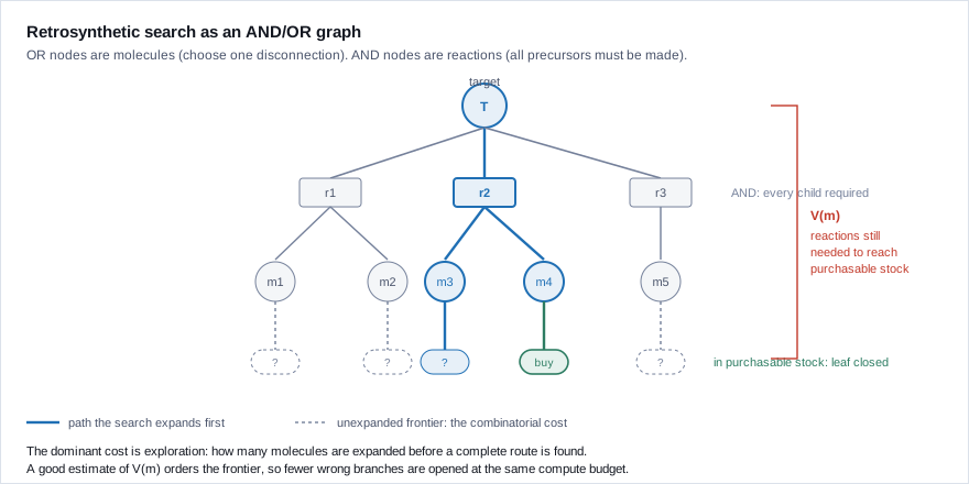
Retrosynthesis is a search over an AND/OR graph. Two kinds of node alternate:
- An OR node is a molecule. To make it you need one of its candidate disconnections, so you may choose whichever looks best.
- An AND node is a reaction. To use it you need all of its precursors, so every child must itself be made or bought.
The search starts at the target molecule and works backwards. A node is closed when the molecule is in a fixed set of purchasable building blocks, called the stock. A route is a subtree in which every leaf is closed.
Formally, write \(\mathcal{R}(m)\) for the set of candidate reactions a one-step model proposes for molecule \(m\), and \(\text{pre}(r)\) for the precursors of reaction \(r\). Define the cost of a route recursively. If \(m\) is in stock, it costs nothing. Otherwise
\[c(m) \;=\; \min_{r \in \mathcal{R}(m)} \Big[\, c(r) \;+\; \sum_{m' \in \text{pre}(r)} c(m') \Big]\]where \(c(r)\) is the cost of running reaction \(r\), often just \(1\) so that the route cost counts reaction steps. The recursion is what makes this an AND/OR problem: the \(\min\) is the OR choice, the \(\sum\) is the AND requirement.
Why the cost explodes
Suppose the one-step model proposes \(b\) candidate reactions per molecule and a typical route is \(d\) steps deep. Exploring the graph exhaustively touches on the order of \(b^{\,d}\) molecules. Even for modest values, say a few tens of candidates and a route half a dozen steps deep, that runs to hundreds of millions of expansions for a single target. No budget covers it.
So every practical planner is a best-first search with a budget. It keeps a frontier of unexpanded molecules, repeatedly picks one, expands it, and stops when a route closes or the budget runs out. The entire quality of the planner reduces to one decision, made thousands of times:
Which molecule on the frontier should be expanded next?
Pick well and a route appears in a few hundred expansions. Pick badly and you exhaust the budget having explored a region of chemistry that was never going to close.
This is the same structure as A* on a road network. There, you order the frontier by
\[f(n) \;=\; g(n) \;+\; h(n)\]the cost already paid plus an estimate of the cost remaining. The estimate \(h\) is the heuristic, and a good one is the difference between a search that finishes and one that does not. In retrosynthesis, \(g\) is cheap to track and the hard part is \(h\).
The quantity that was already there
A planner of the Retro* family already learns something close to \(h\). It trains a value function
\[V(m) \;\approx\; \text{number of reactions still needed to reach purchasable stock from } m\]by regressing on route costs taken from a corpus of known or generated routes. \(V\) is used to order the frontier, which is exactly what A* would do.
But there is a second place a decision gets made, and it is usually made differently. When the planner expands a molecule, the one-step model hands back a ranked list of candidate reactions, and the planner keeps only the top \(k\). That ranking comes from the model’s own likelihood: it scores how plausible each reaction looks on its own.
Plausibility and usefulness are not the same thing. A reaction can be entirely sensible chemistry and lead directly away from anything purchasable. The ranking that decides what survives the cutoff is therefore answering a different question from the one the search cares about.
What I did with it
The diagnostic work pointed at that gap: many reactions a route needs are generated by the model and then discarded because they rank too low. They were never missing. They were thrown away.
The intervention follows directly. Instead of ordering candidate reactions by their own likelihood, order them by the cost-to-go of where they lead:
\[\text{score}(r) \;=\; \sum_{m' \in \text{pre}(r)} V(m')\]A reaction whose precursors are each estimated to be close to purchasable material scores well. One whose precursors are estimated to be far away scores badly, however plausible the reaction looks.
Three properties make this worth doing:
- It costs nothing extra. \(V\) is already trained and already evaluated on these molecules. No new model, no new training data, no extra calls to the one-step model.
- The compute budget is unchanged. The same number of expansions, the same top-\(k\) cutoff, the same candidate generator. Only the order inside the cutoff changes. So any improvement is a navigation gain rather than the result of simply searching more, which is the usual confound in this literature.
- It is a reuse, not an invention. The quantity was designed to answer “how far from stock is this molecule?” and it is being asked exactly that, one level deeper.
Designing an evaluation that cannot flatter itself
The part of this project I would most want to be judged on is not the method. It is the evaluation, because search results in this field are unusually easy to fool yourself with, in ways that are not dishonest.
Three things move the headline solve rate without the search getting any better: changing the candidate generator, changing the stock of purchasable molecules, and evaluating on targets that resemble the training routes. Any of them can manufacture a large improvement.
Four practices did the real work:
An external evaluation set, verified disjoint. The main benchmark and the external set were checked for overlap both exactly and after removing stereochemistry, against the target molecules, every molecule appearing in any route, and the molecules the value function was trained on. Without that check “it generalises” is a hope rather than a measurement.
Paired statistical tests. Comparing two headline percentages tells you almost nothing. Running both methods on the same targets and testing the paired outcomes tells you whether the disagreements are lopsided. For solved-or-not outcomes that is McNemar’s test; for continuous quantities, a bootstrap confidence interval.
Pre-registered run designs. The comparison, the metric, the sample size and what would count as the method not working were committed to the repository before each run and not edited afterwards.
An oracle study to locate the ceiling. Injecting the correct reactions directly tells you how much head-room is left and, more usefully, which component it is in. That answer decided what to work on next, and it was not the component we had been improving.
A control for the obvious confound. The cheapest way to find more routes is to consider more candidates. So that was run as its own arm, to check whether the gain was navigation or just a wider net.
What the evaluation was designed to settle
The results belong to my employer and are not published here. What I can describe is what the design was built to answer, which is the part I would want to be judged on anyway. Each of these was fixed in advance, not chosen after seeing the data:
- Does any improvement come from navigation or from breadth? Settled by holding the candidate generator, the stock and the expansion budget fixed, and running “consider more candidates” as its own separate arm. Without that control a search result is uninterpretable.
- Does it generalise, or does it fit the benchmark? Settled by the external set with the disjointness checks described above. In-distribution improvement on its own establishes nothing.
- Is the difference real or noise? Settled by paired tests on matched targets with confidence intervals, rather than by comparing two headline percentages.
- Where is the remaining head-room, and in which component? Settled by the oracle study. This is the question that decides what to work on next, and the answer was not the component we had been improving.
I will link the published numbers here once the conference abstract is public.
Limitations
Stated plainly, because a result without its limits is advertising.
- The controlled quantity is logical expansions, not wall-clock time. No runtime claim is available from these experiments, and I do not make one.
- The gains are modest and single-run. Multi-seed repetition would turn them into confidence intervals; it has not been done.
- Validated in a backward retrosynthetic planner, not in the complete double-ended system the diagnostic work started from.
- “Solved” means graph closure to a fixed stock. It does not mean the route is synthesisable in a laboratory, which is a stronger and different claim.
- Drug-like targets only. Nothing here speaks to other regions of chemical space.
References
- Retro*: Learning Retrosynthetic Planning with Neural Guided A* Search. Binghong Chen, Chengtao Li, Hanjun Dai, Le Song. ICML 2020. Introduces the neural-guided best-first search over AND/OR graphs, and the learned value function that this work reuses as a reranking signal.
- Double-Ended Synthesis Planning with Goal-Constrained Bidirectional Search. Kevin Yu, Jihye Roh, Connor Coley et al. NeurIPS 2024. The double-ended planner whose architecture the diagnostic phase of this project examined.
- Computer-Assisted Retrosynthesis Based on Molecular Similarity. Connor Coley, Luke Rogers, William Green, Klavs Jensen. ACS Central Science, 2017. Background on template-based one-step retrosynthesis and the ranking problem this work acts on.
- A Note on Two Problems in Connexion with Graphs and the A* literature that follows it. The \(f = g + h\) decomposition, and why the quality of \(h\) decides whether the search finishes.
Related work of mine
The optimization methodology behind this project is public: see Research, and the posts on pre-registering experiments and what a Hessian sketch buys you.