Accelerating Large-Scale Machine Learning: A Deep Dive into SVRG with Barzilai-Borwein Optimization

Gradient noise is the enemy of efficient learning. When you’re training models on millions of data points, mini-batch or stochastic gradient descent (SGD) offers scalability—but at a cost: high variance in updates that leads to slower convergence.

🧮 Objective Functions

This project addresses two main objective functions in convex optimization:

1. L2-Regularized Logistic Regression:

\[\min_w F(w) = \frac{1}{n} \sum_{i=1}^n \log(1 + \exp(-b_i a_i^T w)) + \frac{\lambda}{2} \|w\|^2\]

2. L2-Squared Support Vector Machine (SVM):

\[\min_w F(w) = \frac{1}{2n} \sum_{i=1}^n (\max(0, 1 - b_i a_i^T w))^2 + \frac{\lambda}{2} \|w\|^2\]

and each function can be represent as follows: \(\min_w F(w) = \frac{1}{n} \sum_{i=1}^n f_i(w)\)

Where:

• $a_i \in \mathbb{R}^d$: Feature vector
• $b_i \in { \pm 1 }$: Binary label
• $\lambda$: L2 regularization parameter

In this deep dive, I’ll explore a powerful optimization technique I implemented in MATLAB: Stochastic Variance Reduced Gradient with Barzilai-Borwein as Second-order Information (SVRG-2BB). It masterfully blends concepts from second-order methods and variance reduction to significantly accelerate convergence on critical convex problems like logistic regression and SVMs, particularly relevant in large-scale machine learning.

The proposed serach direction: \(w_{t} = w_{t-1} - \eta\ (\nabla f_{i_t}(w_{t-1}) - \nabla f_{i_t}(\tilde{w}) + \nabla F(\tilde{w}) + {(\tilde{A} - \tilde{A}_{i_t}) (w_{t-1} - \tilde{w})})\)

We choose BB-approximation in following way,

\[\tilde{A}^k = \frac{(s^k)^\top y^\top}{\|s^k\|^2} \mathrm{I} = \frac{1}{n} \sum_{i=1}^{n} \frac{(s^k)^\top (\nabla f_{i}(\tilde{w}_k) - \nabla f_{i}(\tilde{w}_{k-1}))}{\|s^k\|^2},\] \[\tilde{A}^{k}_{i_t} = \frac{(s^k)^\top (\nabla f_{i_t}(\tilde{w}_k) - \nabla f_{i_t}(\tilde{w}_{m-1}))}{\|s^k\|^2},\]

Where \(s^k = \tilde{w}_k - \tilde{w}_{k-1} \text{ and } y^k = \nabla F(\tilde{w}_k) - \nabla F(\tilde{w}_{k-1})\)

Hence, we get

\[\textbf{E}[\tilde{A}_{i_t}] = \tilde{A}.\] \[\tilde{A}_{i_t} \approx \nabla^2 f_{i_t}(\tilde{w}) \text{ and } \tilde{A} \approx \nabla^2 F(\tilde{w})\]

---

🔍 Why Variance Reduction?

In vanilla SGD, the update direction is noisy and fluctuates around the true gradient. This inherent noise can severely impede convergence, especially as datasets grow massive.

SVRG (Stochastic Variance Reduced Gradient) mitigates this by introducing a control variate—effectively anchoring noisy stochastic gradients to more accurate full-gradient snapshots, taken periodically. This intelligent anchoring significantly reduces the variance of gradient estimates.

But there’s more to truly unlocking speed.

---

📈 Adding Barzilai-Borwein: Second-Order Speed for Scalability

While SVRG reduces variance, we can further enhance performance by incorporating curvature information without the computational burden of full Hessian matrices. This is where the Barzilai-Borwein (BB) method comes in—a brilliant step-size heuristic derived from quasi-Newton methods that estimates curvature efficiently.

In SVRG-2BB, we integrate BB into the SVRG direction framework to achieve superior acceleration:

• We utilize BB-approximated step sizes that adapt dynamically within each epoch, leveraging historical gradient information.
• We preserve and enhance SVRG’s core variance-reduction structure, creating a synergistic effect.

The result is better, more stable convergence, particularly on challenging, ill-conditioned problems common in real-world large-scale datasets.

---

🧪 Real-world Example: Gisette Dataset

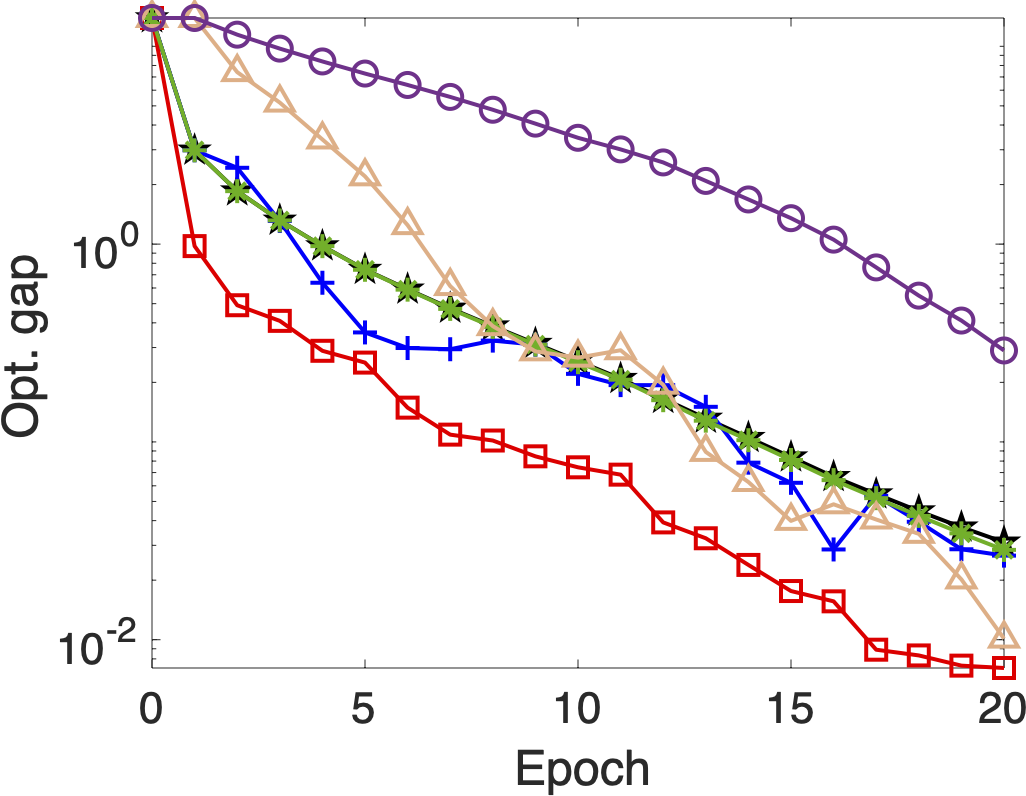
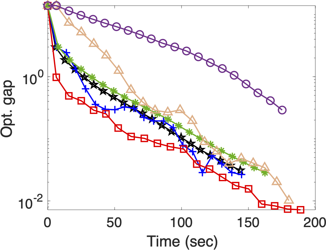
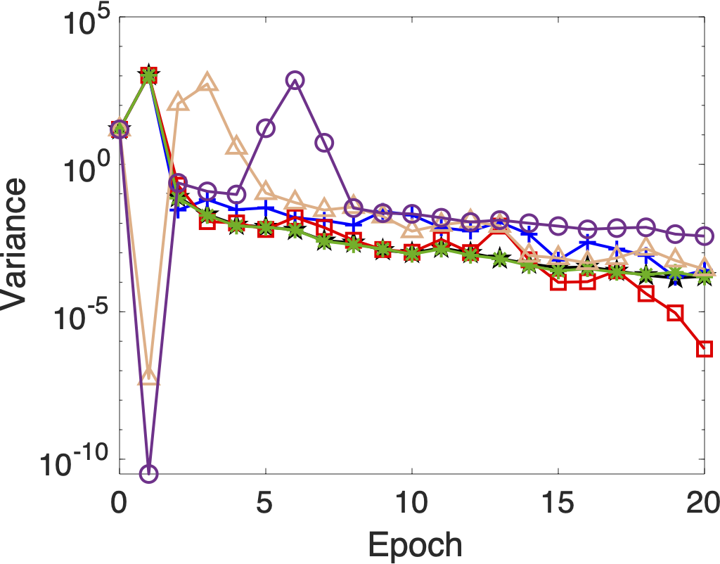
To demonstrate the practical benefits of SVRG-2BB, I evaluated these methods on the Gisette dataset, a well-known challenging high-dimensional classification task. This dataset serves as an excellent benchmark for understanding how optimization algorithms perform under realistic conditions.

Sample Results

• ✅ Optimality Gap vs. Epoch
  A visual representation of how closely the algorithm approaches the true minimum of the objective function as training epochs progress. A faster drop indicates quicker convergence.

• 🕒 Optimality Gap vs. Time
  This plot highlights the real-world efficiency gains. Faster convergence in terms of CPU time translates directly to more efficient model training and quicker iteration cycles in practice.

• 🔁 Variance of Gradient vs. Epoch
  This figure demonstrates how the Barzilai-Borwein steps, when integrated with SVRG, effectively reduce the inherent stochastic noise across iterations, leading to more consistent and reliable updates.

---

💡 Why This Matters for Data Scientists: Bridging Theory and Practice

This approach is not just a theoretical advancement in optimization; it has profound practical applications for data scientists working with large-scale data:

• Large-scale Logistic Regression: Essential for applications like CTR prediction, sentiment analysis, and medical diagnostics.
• Linear SVMs: Effective for spam filtering, image recognition (e.g., OCR), and text classification.
• Any Convex Model: Applicable across a broad spectrum of convex machine learning models where minimizing convergence time is critical.

SVRG-2BB bridges the gap between rigorous theory-driven optimization and the demands of practical, high-performance machine learning workflows, offering a path to build more efficient and scalable solutions.

---

🛠 Try It Yourself

You can explore and run all experiments from this GitHub repo. It provides a clean MATLAB setup for testing various SVRG variants, including the proposed Barzilai-Borwein approximations, allowing you to reproduce and experiment with these powerful optimization techniques.

---

📚 Further Reading

Tankaria Hardik & Yamashita Nobuo A Stochastic Variance Reduced Technique using Barzilai-Borwein techniques as second order information.
Journal of Optimization, Industry, and Management. 2024, 20(2): 525-547